
Spreadsheets “for managers” is a tongue-in-cheek way of saying that none of these features are particularly impressive to have mastered. But, they will help you greatly in almost any knowledge worker role.
This blog post has a companion Google Sheet playground, with examples. Also, I’m not attempting to be exhaustive with any of these topics; merely to provide an introduction and basic syntax examples.
Understanding Cell References
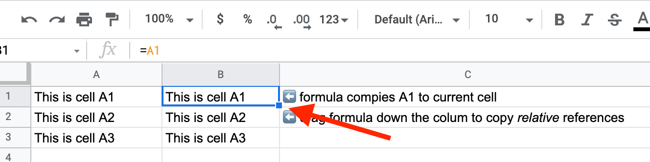
A cell reference in a spreadsheet is a variable that points to another cell. For example formula =A1 would copy the value from cell A1 to the current cell. Bonus: you can give a cell an easy-to-reference name via Data → Named ranges.
Copy Formula
When a range of cells is selected, there is a box handle in the lower right of the range that you can use to copy the formula to other cells. This is mostly used to “fill in” the rest of a column (or occasionally a row) with the same formula.
Note: you can quickly fill the rest of a column with a given formula by holding down COMMAND (on a Mac) and double-clicking on the copy formula box handle. Alternatively, you can script this with ARRAYFORMULA. This is especially useful if you want to automatically apply the formula to new rows in the sheet.
Array formulas should reference entire columns, for example: =ARRAYFORMULA(YEAR(C2:C))
When copying a formula, it’s often useful to keep either the source column number or source row number (or both) fixed. For example, if you are a value in one specific cell, such as the dollar cost average per engineer, you may want to reference that value in another formula. In this case, you would use an absolute reference like $A$1, which would always point to A1, no matter where you copied the formula.
It’s also possible to use a column-relative or row-relative absolute reference, such as A$1 or $A1.
Text Munging
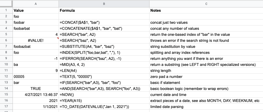
These cover the majority of basic text manipulation.
Official documentation is here:
- CONCAT
- CONCATENATE
- SEARCH
- SUBSTITUTE
- INDEX
- SPLIT
- IFERROR
- MID
- LEN
- TEXT
- IF
- AND
- NOW
- YEAR
- TO_DATE
- DATEVALUE
Honorable mentions: REGEXMATCH, REGEXREPLACE, and COUNTIF.
Import & Export CSV
Spreadsheets allow for easy import and export of CSV data. See File → Import. Importing CSV from some data source, manipulating it, and then doing a pivot table is like 20% of being a manager. 😉
You can use awk, sed, and sometimes just grep to do some basic pre-processing of a CSV file.
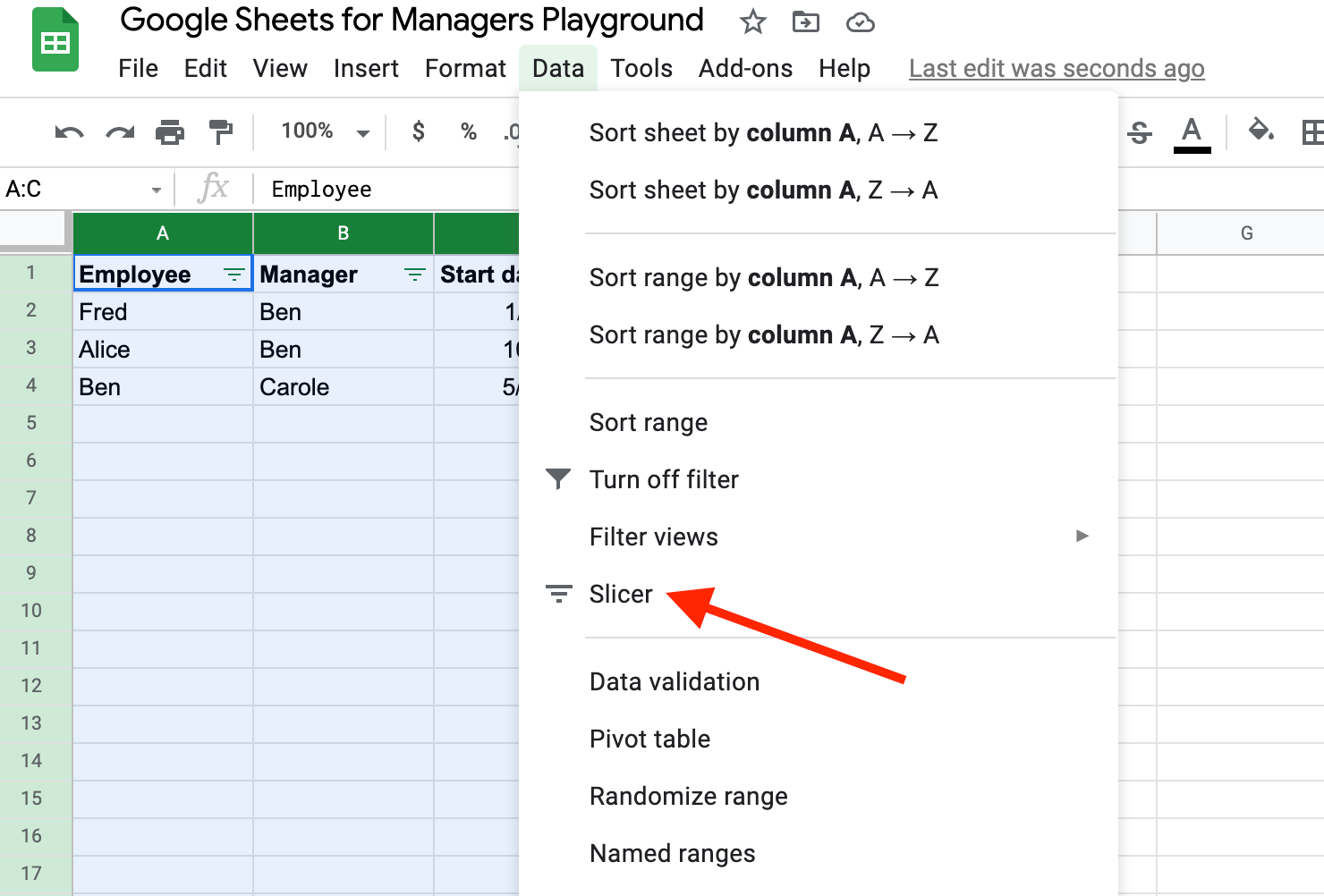
Filters and Slicers
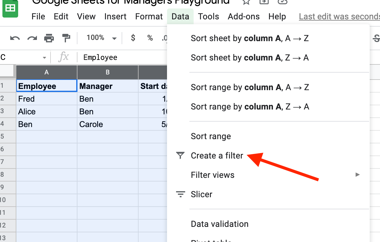
Selecting an entire sheet and doing Data → Create a filter is a handy single-stop shop to a bunch of easy sorting and filtering.
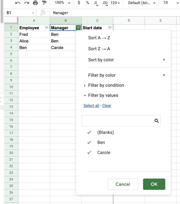
The resulting filters on each column are especially useful for filtering OUT rows that are not relevant. For smallish datasets, you can just un-select the values you want to filter out.
One common issue with filters is that they apply globally to a shared document. This is only what you want about half the time. The rest of the time, you DON’T want a filter that one user applies to their view of the spreadsheet to apply for everyone else. For example, if that user is filtering down to just rows that are relevant to them, such as their direct reports.
In this case, you can use a Slicer to define filters that do not modify the original document for other people.
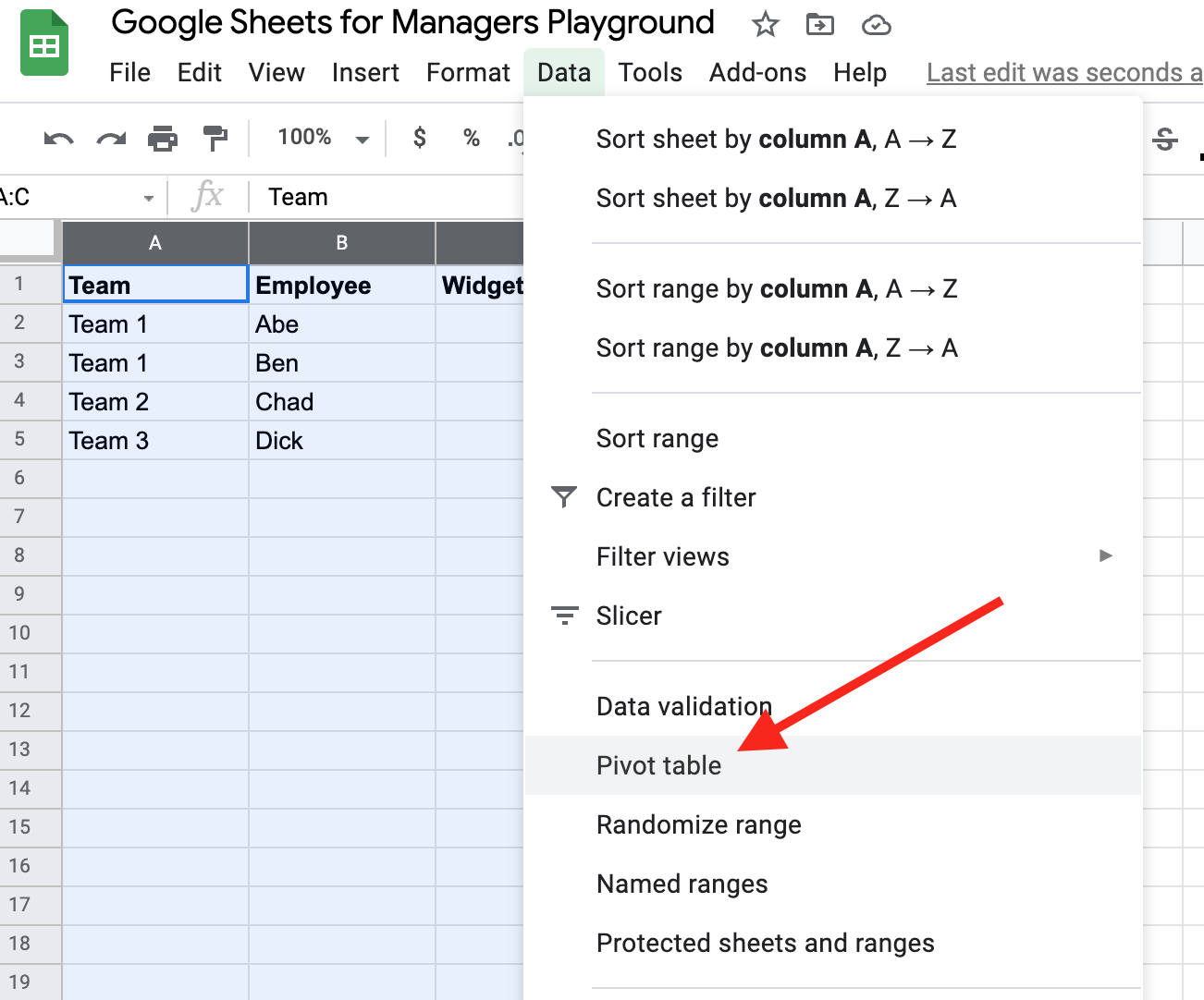
Pivot Tables
Think of a pivot table as a GROUP BY clause in SQL. It’s a general-purpose way to aggregate data and displays things like counts, averages, and sums by one or more dimensions.
First, select the data you want to pivot on and go to Data → Pivot table.
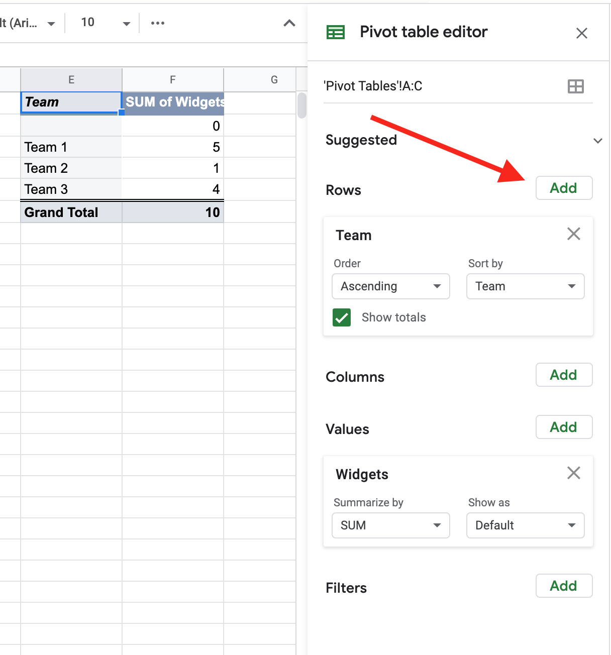
Note: you can make sure that your pivot table will pick up new rows in the source sheet automatically by updating the data range to reference entire columns without specific row numbers, such as A:C. When you do this, you will likely need to add a filter to exclude blank values.
Then use the editor to Add rows and values. Here, I’m summing Widgets by Team.
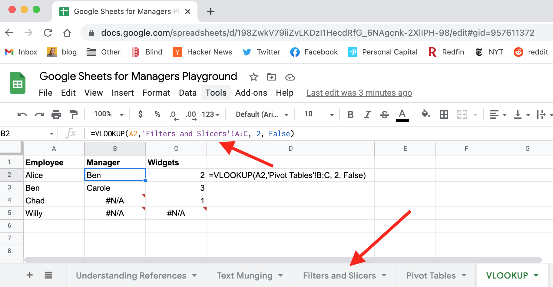
VLOOKUP
If Pivot Tables are analogous to GROUP BY in SQL, then a VLOOKUP is like a JOIN. You can join to data in another sheet in the current Google Sheet document, and you can also join to external sheets.
This is great for at least two use cases:
- You want to treat one sheet as a source-of-truth enum-like mapping, i.e. a translation table.
- You want to reference another dataset either to not repeat data or because you know that the source-of-truth sheet will change regularly, i.e. a list of employees and their current manager.
Note: I always have to look up the syntax of this, and do some debugging. 😉 The key is to remember that you’re looking up the value in the first column of the range.
The arguments of the vlookup function are:
- The value to search for, i.e.
A1 - Where to do the lookup, again it’s going to look at the first column in this range
- You can provide a range in the local sheet like
A:C - You can provide a range in another sheet in the current document like
'Filters and Slicers'!A:C(you must use single quotes if the name of your sheet contains spaces) - You can provide a range in another Google Sheet document like
importrange("https://docs.google.com/spreadsheets/d/1YH6-gXcIix5Pql97nqVaENxN8rUbL-JarOrpnH9DNZT0/edit#gid=1511625096","employees!A:G")
- You can provide a range in the local sheet like
- The index of the value in the range to return. If you find yourself wanting to return a value with a negative index (i.e. to the left of the range), you can instead change the range to an array where you reorder the columns. For example: instead of
A:C, use{'Filters and Slicers'!C:C,'Filters and Slicers'!A:A}. - Returns exact matches only when set to
False(you probably want this)
Conditional Formatting
Conditional formatting is just styling cells based on their contents.
Common use cases:
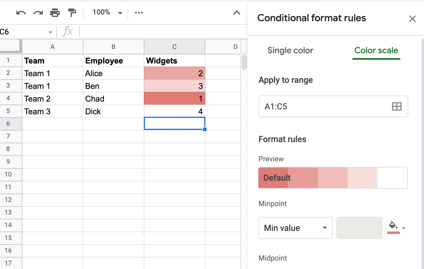
- Use background color as a heat map to denote high/low values
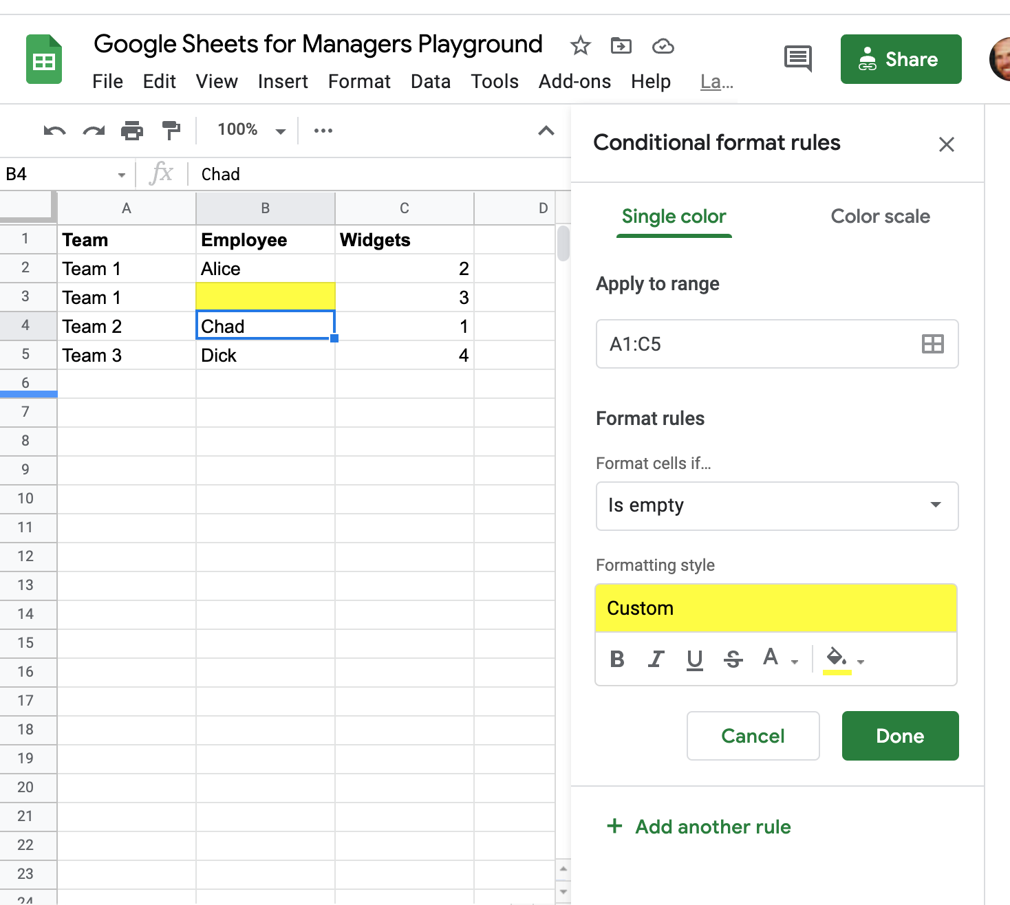
- Use background color to highlight rows that are not filled out, i.e. you’re asking others to fill them in
- Alternating row background colors for readability
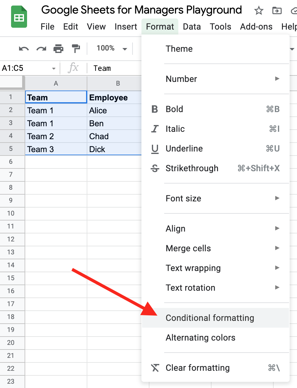
Start by selecting a range, and going to Format → Conditional formatting
Example of highlighting empty cells:
Example of a heat map:
Conclusion
If you use a tool long enough, you may begin to assume that everyone knows it as well as you do. I’m certainly not a spreadsheet master, but I’ve come to realize that some people barely use them at all. For me, they are the primary tool I turn to in many different contexts. It’s been said that spreadsheets could perform the function of 80% of custom software, and I would agree. For me, basic functional spreadsheet knowledge is right up there in terms of utility with writing SQL, or coding itself.